SQL_Exploratory

Create table

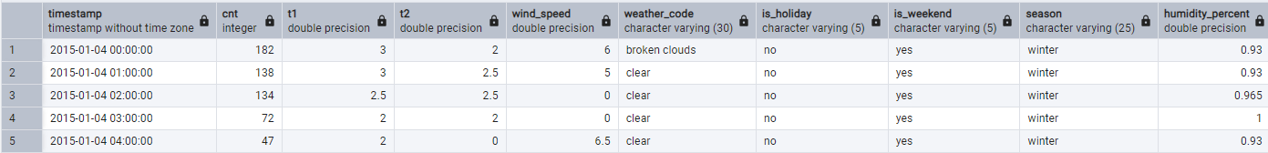
CREATE TABLE bike_sharing (
    timestamp TIMESTAMP,
    cnt INTEGER,
    t1 FLOAT,
    t2 FLOAT,
    wind_speed FLOAT,
    weather_code VARCHAR(30),
    is_holiday VARCHAR(5),
    is_weekend VARCHAR(5),
    season VARCHAR(25),
	humidity_percent FLOAT
);

Verify table exists in PostgreSQL

SELECT * 
FROM bike_sharing
LIMIT 5;

Business Questions

1. What is the start and end date and duration of bike rental tracking in our data?

SELECT
 MIN(timestamp :: DATE) AS starting_date,
 MAX(timestamp :: DATE) AS end_date,
 (MAX(timestamp :: DATE) - MIN(timestamp :: DATE)) AS days_tracked
FROM bike_sharing;

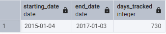
Insight: The dataset encompasses a full two-year period, from January 4, 2015, to January 3, 2017, providing 730 days of data. This comprehensive timeframe is robust enough to identify and analyze daily, weekly, and seasonal ridership patterns with confidence.

2. What is the total amount of bike rentals during the 730 days?

SELECT
 SUM(cnt) AS total_bike_rentals
FROM bike_sharing;

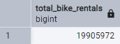
Insight: Over the two-year period, nearly 20 million bike rentals were recorded. This substantial volume underscores the service's significance as a major component of London's public transport system and highlights the scale of the operational challenge.

2.1 What is the total amount of bike rentals per year?

SELECT
 EXTRACT(Year FROM timestamp) AS bs_year,
 SUM(cnt) AS bike_rentals_per_year
FROM bike_sharing
GROUP BY 1
ORDER BY 1;

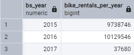
Insight: The analysis shows a positive year-over-year growth in ridership from 2015 to 2016. The low rental count for 2017 is expected, as the dataset only includes the first three days of that year and does not represent a full year's performance.

3. What are the top 5 days with the highest number of bike rentals?

SELECT
 timestamp :: DATE,
 TO_CHAR(timestamp :: DATE, 'Day') AS weekday,
 SUM(cnt) AS daily_bike_rentals
FROM bike_sharing
GROUP BY 1,2
ORDER BY 3 DESC
LIMIT 5;

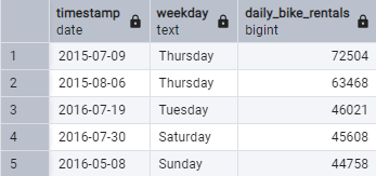
Insight: The days with the highest rental counts are concentrated in the peak summer month of July. This strongly suggests that a combination of factors—warm weather, longer daylight hours, and potentially public events or holidays—creates days with exceptionally high demand. The top day, July 9th, 2015, saw over 72,000 rentals, serving as a benchmark for maximum operational capacity.

4. What was the most popular season for bike rentals in each year?

SELECT
 bs_year,
 season,
 bike_rentals_per_year
FROM(
 SELECT
  EXTRACT(Year FROM timestamp) AS bs_year,
  season,
  SUM(cnt) AS bike_rentals_per_year,
  RANK()OVER(
    PARTITION BY EXTRACT(Year FROM timestamp)
    ORDER BY SUM(cnt) DESC
  ) AS rnk
  FROM bike_sharing
  GROUP BY 1, 2
)
WHERE rnk = 1;

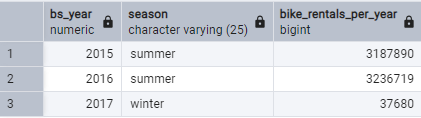
Insight: Summer was consistently the most popular season for bike rentals in both full years of data (2015 and 2016), reinforcing the strong link between warmer weather and higher ridership. The result for 2017 reflects only the first few days of January, which fall in winter.

5. Show the minimum, average and maximum actual daily temperatures.

SELECT
	timestamp::DATE AS bs_date,
	MIN(t1) AS min_daily_temp,
	ROUND(AVG(t1):: NUMERIC, 1) AS avg_daily_temp,
	MAX(t1) AS max_daily_temp
FROM bike_sharing
GROUP BY 1
ORDER BY 1;

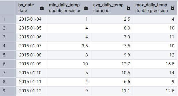
Insight: This query transforms the hourly data into a daily summary of temperature ranges. This aggregated view is essential for analyzing macro trends, as it allows us to correlate overall daily rental volumes with average temperatures and understand the impact of temperature fluctuations throughout a single day.

6. What are the humidity levels at which the maximum and minimum number of bike rentals occurred?

WITH rental_count_humidity AS (
 SELECT 
  humidity_percent,
  SUM(cnt) AS total_bike_rentals
 FROM bike_sharing
 GROUP BY 1
)

SELECT *
FROM rental_count_humidity
WHERE total_bike_rentals IN (
 SELECT 
  MAX(total_bike_rentals) AS max_rentals
 FROM rental_count_humidity
 UNION
 SELECT
  MIN (total_bike_rentals) AS min_rentals
 FROM rental_count_humidity);

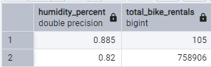
Insight: This query reveals an interesting paradox: both the highest and lowest total rental volumes occurred at very high humidity levels (82% and 88.5%, respectively). This suggests that while extreme humidity can be a deterrent, it is not the sole factor. The day with the highest volume (758k rentals at 82% humidity) was likely driven by other powerful factors like ideal temperature and a special event, which were strong enough to overcome the discomfort of the high humidity.

7. Find the 7-day moving average for total bike rentals

WITH daily_rentals AS(
SELECT
 timestamp :: DATE AS bs_date,
 SUM(cnt) AS total_bike_rentals
FROM bike_sharing
GROUP BY 1
ORDER BY 1
)
SELECT
 bs_date,
 total_bike_rentals,
 CASE WHEN ROW_NUMBER()OVER(ORDER BY bs_date) < 7 THEN NULL
 ELSE ROUND(AVG(total_bike_rentals) OVER(
  ORDER BY bs_date
  ROWS BETWEEN 6 PRECEDING AND CURRENT ROW
  ), 2) END AS seven_day_moving_avg
FROM daily_rentals
ORDER BY 1;

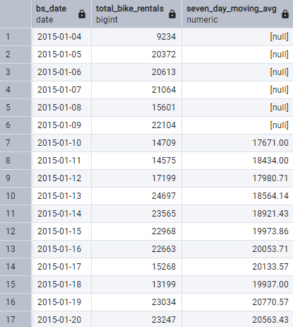
Insight: By calculating a 7-day moving average, we can smooth out daily fluctuations and better identify the underlying weekly trends in ridership. This technique is crucial for distinguishing genuine shifts in demand from random daily noise, enabling more accurate medium-term forecasting and resource planning.

8. How do weekends and holidays influence bike rental volumes compared to weekdays?

WITH day_type_rental_counts AS (
 SELECT 
  SUM(CASE WHEN is_weekend = 'yes' THEN cnt ELSE 0 END) AS weekend_rentals,
  SUM(CASE WHEN is_holiday = 'yes' THEN cnt ELSE 0 END) AS holiday_rentals,
  SUM(CASE WHEN is_weekend = 'no' AND is_holiday = 'no' THEN cnt ELSE 0 END) AS weekday_rentals,
  COUNT(DISTINCT DATE_TRUNC('day', timestamp))FILTER(WHERE is_weekend = 'yes') AS weekend_days,
  COUNT(DISTINCT DATE_TRUNC('day', timestamp))FILTER(WHERE is_holiday = 'yes') AS holiday_days,
  COUNT(DISTINCT DATE_TRUNC('day', timestamp))FILTER(WHERE is_weekend = 'no' AND is_holiday = 'no') AS weekday_days
 FROM bike_sharing
)

SELECT 
 weekend_rentals / weekend_days AS avg_weekend_daily_rentals,
 holiday_rentals / holiday_days AS avg_holiday_daily_rentals,
 weekday_rentals / weekday_days AS avg_weekday_daily_rentals
FROM day_type_rental_counts;

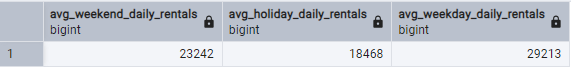
Insight: On an average day, weekday rental volume (29,213) is significantly higher than on weekends (23,242) and holidays (18,468). This quantifies the usage difference, showing that an average weekday is approximately 26% busier than an average weekend day, confirming that the service is driven primarily by commuting rather than leisure activities.

9. Write a query to classify the days into "High Traffic" (if cnt > 90th percentile), "Medium Traffic" (between 50th and 90th percentile), and "Low Traffic" (below the 50th percentile).What percentage of the dataset falls in the high traffic category?

WITH percentile AS (
  SELECT 
    PERCENTILE_CONT(0.50) WITHIN GROUP (ORDER BY cnt) AS pctile_50,
    PERCENTILE_CONT(0.90) WITHIN GROUP (ORDER BY cnt) AS pctile_90
  FROM bike_sharing
)
SELECT 
 ROUND(
   (SELECT 
     COUNT(*) 
   FROM (
     SELECT
       timestamp :: date AS dt,
       cnt,
       CASE
         WHEN cnt > (SELECT pctile_90 FROM percentile) THEN 'High Traffic'
         WHEN cnt <= (SELECT pctile_50 FROM percentile) THEN 'Low Traffic'
         ELSE 'Medium Traffic'
       END AS traffic_lvl
       FROM bike_sharing
       ) AS traffic_data
       WHERE traffic_lvl = 'High Traffic')::numeric / (SELECT COUNT(*) FROM bike_sharing)::numeric * 100, 3) AS high_traffic_percentage;

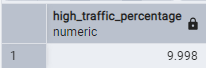
Insight: By segmenting hourly data into traffic tiers based on rental volume percentiles, we find that only the top 10% of hours qualify as "High Traffic." This confirms that peak demand is highly concentrated in specific, predictable periods (like commuter rush hours), making it crucial to focus operational resources on these critical windows to maximize service availability and revenue.

London bike sharing EDA 🚲